Measurement of Multidimensional Brand Loyalty of a Consumer

Recently the author presented a factor analytic model with loyalty scores of individual consumers to a brand [6]. This paper is an extension of the model to a more realistic situation in which a consumer has varying degrees of loyalty to several brands.

Obviously, a buyer is loyal not only to one brand but to many brands in the market, although he may have greater loyalty to one particular brand over others. In theory, he has scene loyalty score for each of the brands that he is aware of, including a zero score for a large number of them. Non-zero loyalty scores indicate his narrowing choice to brands he considers buying (his evoked set) from among those of which he is aware, and these are often a small subset of existing brands.

Second, research on buyer attitudes is usually carried Out on several brands in the market because there is a built-in hypothesis that the buyer has, in fact, a rank order of preferences, because he prefers some brands more than others. However, in research on buyers’ overt behavior, this multidimensionality of preferences (projection of loyalty to brands on a multidimensional space in which each dimension represents a brand) is not emphasized to the same extent. See [2, 5] for reviews of studies. Some promising ramifications of measures of aggregate loyalties for market shares are in [3]. ¹ This article attempts:

1. To provide robust measures of multidimensional brand loyalty of each consumer in which each dimension is a brand specified in analysis. In other wards if a buyer is loyal to more than one brand, his brand loyalty is a point in space of n dimensions rather than unidimensional, n being the number of brands.

These measures may be time-independent or dependent, probably depending upon the product life cycle and the time period under observation and analysis. For example, following statistical learning theory, new products may manifest time-dependent loyalty, but as they become well established and mature, a consumer may buy because of habit learned from past purchase experiences.

In time-independent situations, measuring a consumer’s multidimensional brand loyalty seems relatively simple, because the relative frequencies of purchase of a particular brand out of total purchases during some specified time period provide a good measure. However, in time-dependent situations this is difficult because stochastic approaches have been oriented toward aggregate (not individual buyers) behavior. Attempts have been made in psychology to use stochastic models, specifically for an individual, but the procedures are essentially judgmental and cumbersome [1]. Furthermore, most work in marketing is still empirical and inductive, and there is not enough known about a market to specify a priori whether a consumers loyalty to a brand is time-dependent or not. The method utilized in this article is general enough to handle both types of phenomena.

2. To discus measures of market shares in which sales to individual consumers are weighted by the relative strengths of brand loyalty.

Description of the Factor Analytic Model

The mathematical aspect of the factor analytic model of brand loyalty was described in an earlier paper [6]. It is a type of factor analysis which gives a least squares solution to a data matrix. The data matrix is created so that (1) it expresses a buyer’s consecutive purchases as a function of trials or time periods, and (2) it preserves information about level and dispersion in addition to shape and so generates a cross-product instead of correlation matrix.

This article will, however, discuss the rationale for using factor analysis, the steps involved in preparation of the input date matrix to obtain the multidimensional brand loyalty scores of a buyer, and the implications of loyalty scores for measurement of aggregate market shares.
In factor analysis, a factor F is a hypothetical index- type construct which is created by a linear combination of the manifest variables. Thus,

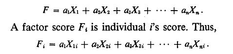
Finally, the factor loadings (related to the weights used in making linear combinations) are the correlations between the factor scores and the manifest scores.

This description of factor analysis makes it similar to multiple regression, in which the estimated values of the criterion variable (y) are created by a linear combination using the rule of least squares. The difference between the two lies in the fact that in factor analysis there is no manifest data on the Criterion variable, F.

Depending on correlations among the manifest variables, several factors are usually derived in factor analysis, each of which is an orthogonal dimension. If each factor (dimension) is looked upon as representing a brand loyalty axis, a buyer’s loyalty toward several brands is a point in space defined by these factors.

Suppose a consumer has this purchase pattern during some specified time period: B,C,C,A,B,AA,A. Of a total of eight purchases, four relate to Brand A and two to each of two other Brands, B and C. Each purchase trial can be considered a manifest variable (X, j = 1,2,3, 8) which can take on binary values: one ii it is a purchase of Brand A and zero if it is a purchase of not-A, either B or C in our example. By labeling the eight trials consecutively (X1 = first trial and X8 = last trial), the time dimension is brought in. f he eight manifest variables can now be combined line by providing weights, say the ratio of one purchase to all purchases, or 1/8 . Then, following the previous discussion, this buyer’s factor score is shown in the following linear combination:

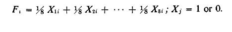
In the example, this score comes to 4/8 = .50, which the relative frequency of purchase of A. This factor ‘core is thus an expression of the buyer’s strength of loyalty to Brand A. Note also that equal weights are specified for each of the trials, to express the assumption of independence of path (time).

Suppose, however, that strength of brand loyalty is an increasing function of trials. Then the weights (a1) are set so that a1 <a2 <a3 <…. <a8. The weights’ relative differences then specify the particular mono- tonic increasing function; if the first differences are identical, then the strength of brand loyalty is a linearly increasing function of trials and similar to a first-order Markov process with constant transitions. If the first differences of the weights are not identical, then brand loyalty is a more complicated (and probably a nonstationary first-order or even a higher-order Markov) function of trials. These weights can be plotted on a graph with trials on the independent axis to show the relations hips in the above situations. This, then, is the rationale for using factor analysis to derive the weights and for calling factor scores brand loyalty scores.

By considering each trial itself as multidimensional, in which each brand is a dimension, loyalty scores for all brands (not just a particular brand) can be derived. This is equivalent to the treatment of brands as states in stochastic models. However, in this case, these brands need not be mutually exclusive and exhaustive, although in the case of trial-by-trial .analysis it is generally the case. If the analysis, however, is such that the time dimension is specified not by consecutive trials but by consecutive, equally spaced time intervals, such as a week or a quarter, then this restriction is not realistic for a number of product categories in grocery foods. For example, multiple purchases of cold cereals, frozen orange juice, or even coffee are quite common. The method discussed here can be useful in these product categories.

In the above example, however, each trial consists of these mutually exclusive and exhaustive dimensions (brands). Then there is a total of 24 manifest variables (Xn = 24) in which each trial is considered as a three- dimensional variable. Each variable will contain the binary information of one if the brand represented by that variable was purchased in that trial, or zero if otherwise.

Steps Involved In Analysis

The particular type of data analysis proposed in the factor analytic model of brand loyalty uses the Eckart Young theorem of approximating a data matrix X with another matrix X of a considerably lower rank, in which this approximation is based on the least squares principle. It is necessary to set up the data matrix from raw data in a specific way to use this theorem meaningfully. This procedure is not complex and, in fact, requires less transformation of raw data than in the standard R-type factor analysis where raw scores are converted into standard scores from which a matrix of simple correlations is created. The steps are described below with the use of a simple hypothetical example.

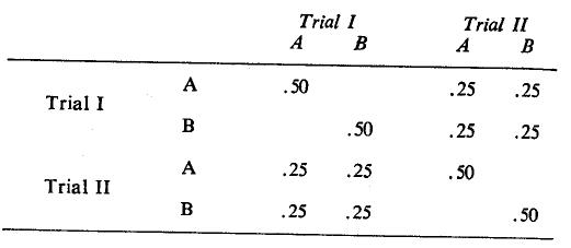
Suppose four consumers each made purchases two times, and each time the choice was between Brands A and B. Each trial (purchase incident) is a two-dimensional variable. Hence, there are four variables (2 trials x 2 brands). A data ma&ix of all four consumers is as follows:

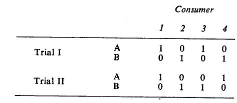
In this matrix, each cell has a value of one if a consumer bought a brand in a particular trial, and a value of zero if otherwise. Thus, from the data the first two consumers are obviously loyal to Brands A and B, respectively, because they continued to buy the same brand, whereas the last two consumers are not loyal to either because each switched to the other brand.

The first step is to produce the cross-products of this matrix X by post-multiplying it by its transpose X’. The results are given below:

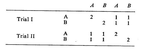
This is a square symmetric matrix similar to a correlation or covariance matrix, and it can be seen as a manifold contingency table [8], which provides joint absolute frequencies over trials, It is actually a super- matrix in which the diagonal matrices contain values only in the diagonals, because each trial has two mutually exclusive and exhaustive brands as dimensions. Furthermore, the diagonal matrices contain absolute frequencies of purchase of each brand in each trial, and the off-diagonal matrices contain the absolute frequencies of brand staying and brand switching between trials. In the example, each brand was bought by two consumers in each of the two trials. Out of the two consumers who each bought a brand, one switched to the other brand in the next trial.

To digress somewhat, equal-interval time periods can be used to create a data matrix of the above type in which cell values represent absolute incidents of purchases of each of the brands in the analysis. Because a buyer may have purchased more than one brand during the time period, the cross-products of the data matrix may contain values in cells other than the diagonal in the diagonal matrix. However, the cross-products matrix is still a square symmetric matrix permitting the use of Eckart-Young theorem. Also, instead of just purchase incidents, the volume of purchase at each incident could be incorporated, which gives more realistic measures at market shares.
Returning to the example, the absolute joint frequencies (as above) are also partially determined by the sample size, so that two identical patterns of purchases differing in sample size will yield different results. It is desirable to transform absolute frequencies into relative ones by dividing each cell value by the sample size, N. The following are results:

This standardized cross-products matrix becomes the input to factor analysis. However, often it is desirable to equalize standard deviations among variables: (1) to remove differences in standard deviations between brands and (2) in situations where some of the dimensions may be added subsequently to later trials (new brand is introduced after two trials in a ten-trial Sequence) or deleted from them (a brand is withdrawn from the market during the last four trials in a ten-trial sequence). This is done by dividing the relative frequencies by their standard deviations. With this further transformation, the square symmetric matrix contains ones in the diagonals and proportionate values in the off-diagonal matrices. It now resembles a correlation matrix, and the interpretation of factor loadings becomes easier.

Factoring of the standardized data matrix results in a set of factors with loadings on the variables and corresponding factor scores for consumers in the analysis. Since factor scores are linear combinations of manifest purchase patterns, they are thus brand loyalty scores. The weights derived in making these combinations: (1) are optimal in the sense that they explain the largest variance in the data matrix and (2) have relative values as well as the first and higher differences between consecutive weights to show whether loyalty to various brands is time-dependent or not.

Such factor analysis of a data matrix gives the following results. First, if each brand in the market has its own segment of buyers who never switch, there should be as many factors as there arc brands, irrespective of the length of analysis. Also, since there is no gain or loss from other brands, there is a steady state or equilibrium so that the weights for each brand will be constant over trials. Second, the alternative possibility is complete, random brand switching from trial to trial. In this case, there should be as many factors as variables, suggesting uniqueness of each brand at each trial. Both of these situations are extremes unlikely to exist in reality. A ….

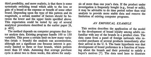
measurement of multidimensional brand loyalty came from the first four purchases of rice by 21 panel members. At the end of five months, these members bought two major brands of rice, Sultana (S) and River (R), as well as a number of other national and private label brands, which were recorded in the diaries. These were small enough in number to lump together as Others (O) in the analysis. ²

The data matrix X then consists of 12 row variables (3 brands times 4 trials) and 21 columns representing purchase patterns of the panel members. The first step is to create the cross-products matrix XX’ by post- multiplying X by its transpose, as in Table 1. It is a square symmetric super-matrix with four diagonal matrices, for each trial, which summarizes the absolute frequencies of purchase of brands at each trial. The off- diagonal matrices summarize the absolute joint frequencies across trials. For example, all six consumers buying Brand S at the first trial continued to buy it at the second, but one of them switched to Brand 0 at the third and continued to buy it at the fourth. Brand-switching seems greater in the case of Brand K than Brand S. Table 1 suggests that on the whole most consumers continued to buy their first brand. Thus factor analyzing the data reveals three dominant factors, each representing a brand.

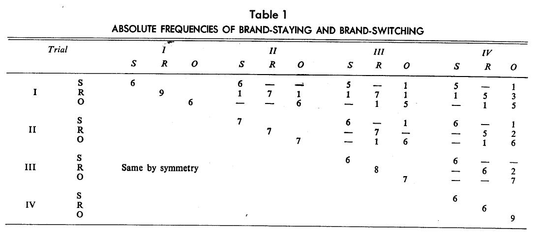
The cross-products matrix in Table 1 was standardized to remove sample size bias. The resultant matrix, say R, is presented in Table 2. Dividing the relative frequencies by their standard deviations gives unity in the diagonals and proportionate values in the off-diagonal matrices, as discussed earlier. The earlier finding of very limited brand switching is even more dramatically seen in the values of the brand-staying and brand-switching cells in the off-diagonal matrices.
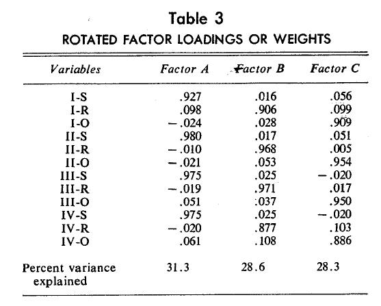
The standardized data matrix R was factor analyzed (following the procedures in [6]). The first three factors explained nearly 90% of the variance in the data, but the fourth and subsequent factors explained individually at best three percent. The factors were rotated using simple structure principles of Varimax rotation to simplify factors instead of variables, in line with the objective of obtaining multidimensional brand loyalty scores for individual panel members. Table 3 shows the rotated factor loadings. It is obvious that each factor represents one brand state and shows that the extent of brand switching in the data is limited enough to warrant no additional factors shared by more than one brand.

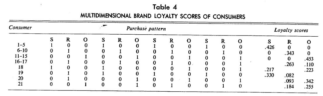
Loyalty scores of each panel member corresponding to the three brand dimensions were calculated. They are reproduced in Table 4. For clarity, Table 4 groupings arc according to similarity of purchase patterns. The first five bought Brand S only, the next five bought Brand 0 only, and the next five consumers bought Brand K only. Accordingly, the first 15 consumers have non-zero values toward one brand only; their brand loyalty is unidimensional.

In contrast, the last six have multidimensional brand loyalty scores because they switched brands during the four-trial sequence. Their loyalty scores are directly a function of the frequency and pattern of purchase sequences.

Comparison of Loyalty Scores with Probability Measures

Comparing the multidimensional loyalty scores with the probabilities of specific brand purchases is not difficult for the first 15 consumers since they all purchased only one brand, The last six consumers become the focus of discussion.

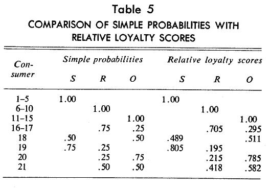
Probability estimates of purchase of a brand calculated Irons the relative frequencies are provided in Table 5. Multidimensional brand loyalty scores are converted into relative scores by taking the ratio of a brands score to a consumer’s total scores. For example, Consumer 16 has two-dimensional values of .263 and .110, so his probability of buying Brand R is .263/(.263 + .110) = .705 and of buying Brand 0 is .295 or 1 — .705. This seems appropriate because brand loyalty scores are themselves based on the frequency and pattern of purchases. These relative scores are also given in Table 5 along with the simple probabilities.

The relative scores systematically deviate from simple probabilities. For example, Consumer 16’s probabilities sad relative scores and their deviations appear to be functions of the brands involved (Brand 0) in switching. Consumers 18 and 21 have identical patterns of brand switching, but the brands involved are S and O in the first case and O and R in the second. However, the deviations toward the brand they switched to are different (.011 as compared to .082).

How can this be explained? Obviously, it suggests that the weights used in making linear combinations are not equal between the two patterns. More importantly, it can be shown that the disproportionate weights are themselves based on only the relative strengths of brand attraction (gain) and defection (loss) in the example because coincidentally the same number of consumers (five) bought the three brands exclusively. It should be pointed Out that in other circumstances, the disproportionate weights between brands would be a function of both the number of loyal customers and the trade-off between gains and losses.

Measurement of Weighted Market Shares

Multidimensional loyalty scores are potentially useful in redefining market shares. The usual accounting- oriented method is to calculate the relative volume or frequency of purchase of a brand in the market out of the total volume or frequency. What is done, of course, is the equal aggregation of the purchases of loyal and nonloyal customers within a certain time period. Managers, however, need to calculate market shares with a weighted aggregation of loyal and nonloyal customers, the weights differentiating them in some manner. This is a useful concept because, first, a company today seeks optimization of long-term profits; this makes the common measures of market shares incompatible. Second, the marketing manager attempts to derive a marketing mix which will create satisfied customers who will buy repeatedly. Otherwise, most of the promotional costs, Such as free sampling, arc not justifiable. Both of these points demonstrate that a loyal customer should somehow be given greater importance or weight to reflect the reality of today’s marketing practices.

Simple market shares can be easily calculated from the data by taking the relative frequencies of a brand out of a total of 84 purchases (4 trials x 21 consumers). The market shares are then: Brand S = .30; Brand R = .36; Brand 0 = .34.

Multidimensional loyalty scores are essentially frequencies weighted by degree of switching. Weighted market shares for each brand are calculated by summing loyalty scores over individuals and diving this by the total sum of scores for all the brands:

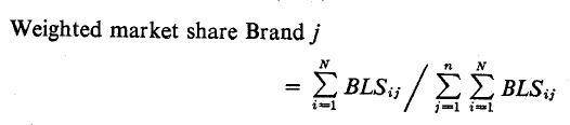
Where BLSij = brand loyalty score of Consumer i for Brand j, N = sample of consumers in analysis, and a = number of brands in analysis.

The weighted market shares of the three brands are: Brand S = .31; Brand R = .31; Brand O = .38.
Compared to simple market shares, Brand R seems to have suffered most by losing five percentage points of its market share which represent, of course, the total gains to other brands. Furthermore, most of the gain is experienced by Brand 0 (4 Out of 5 percentage points). Since the number of fully loyal customers is the same for all the three brands, the differences between the simple and the weighted market shares are a function of the brand switching in the data.

Focusing attention on Brand R, the picture looks good if the simple market share measure is used as the criterion for evaluation; it is the brand with largest market share and perhaps correspondingly good profits for the time period under investigation. However, the picture changes if the weighted market share is used as the criterion of evaluation because it clearly indicates to management that market is not unsteady and loyal for its brand.

Implications for Research

A number of implications seem to flow from the fact or analytic model Broadly, they relate to three issues.

First, and perhaps the most important implication is that more robust measures of an individual buyer’s brand loyalty to various brands in the market are obtained. These multidimensional loyalty scores also incorporate time dependencies in the data if they exist. Such measures are of considerable importance in test marketing new products, because time dependencies generally exist between marketing activities and the adoption of new products. Aggregate simple market share measures are often misleading because time allotted to test market a new product is still judgmental and arbitrary. In addition, the multidimensional loyalty scores summarize succinctly the individual’s brand staying and brand switching behavior, from which one can find out relatively easily where the market is coming from (or the new product. Using loyalty scores for segmentation helps isolate those consumers attracted to the new product and study them more carefully with respect to their socioeconomic and psychological profiles.

Second, the multidimensional brand loyalty scores seem to provide a much better measure of brand loyalty as the criterion variable. Too little attention has been paid to the adequacy of the dependent variable in marketing research. This has led marketers to believe that many of the personality, psychological, or socio economic predictor variables are of little significance in predicting brand loyalty or buyer behavior. The brand loyalty scores are mostly empirically derived, with time dependencies, if any, adequately summarized. To that extent they contain fewer assumptions than a researcher may have to make when he attempts to fit a model (e.g., Markov chains) to the data. As such, loyalty scores seem more representative of reality.

Finally, the derivation of weighted market shares can be extended to include purchase measures other than the incidence of purchase which was used in this article. For example, volume or units purchased at each trial oe during some time interval can be used in the model if that is more appropriate to a given industry. The model can be used with a variety of input data depending upon the needs of the industry. Furthermore, as mentioned earlier, the model is capable of giving weighted market shares for those industries where multiple purchases by consumers are common, as for example, in cereals, juices, toothpaste, and even coffee.

References