Multivariate Analysis in Marketing

Formerly expensive, exotic and ill-understood, today most analytic methods have–thanks to computers–become affordable and commonplace. Here is a readable review of Multivariate Analysis of Marketing Data

[button open_new_tab=”true” color=”accent-color” hover_text_color_override=”#fff” image=”default-arrow” size=”large” url=”https://www.jagsheth.com/wp-content/uploads/2015/12/Multivariate-Analysis-in-Marketing.pdf” text=”View Original Article” color_override=””]

Reading the history of disciplines, it appears that every discipline experiences two things during its transition from a speculative philosophy to a branch of empirical science. First, it begins to apply and generate certain statistical techniques. Second, it seeks guidance from more mature disciplines in applying statistical models. Both psychology and economics, for example, went through this process recently in which they sought guidance from mechanics and chemistry. Unfortunately, this Imitative tendency creates overabundance and overemphasis of some special statistical models. In the case of both psychology and economics, for example, bivariate analysis received greater attention because that was all that both mechanics and chemistry could offer. This explains to a large extent relatively recent application and development of multivariate techniques in psychology despite the fact that one of the first persons to point out the need for multivariate analysis in social sciences was Galton.

Currently, marketing seems to be in the transition period from speculative thinking to empirical research [96]. It is, therefore, not surprising to observe that most articles in marketing journals today either apply known statistical techniques or generate some new ones especially suited to marketing research. Perhaps the greatest proliferation seems to be the application of multivariate techniques. There are two reasons. First, marketing seeks guidance from psychology and economics both of which currently offer a variety of multivariate methods. Second, in an effort to segment market based on individual differences, marketing researchers agree that consumer behavior and marketing environment surrounding him are complex enough to make univariate or bivariate analysis inadequate. Indeed, this thinking goes to far as to state: “For the purposes of marketing research or any other applied field, most of our tools are, or should be, multivariate. One is pushed to a conclusion that unless a marketing problem is treated as a multivariate problem, it is treated superficially” [42, p. 158].

In light of the current interest in and emphasis on multivariate analysis, this paper attempts to non-technically describe some of the multivariate methods, review existing applications in marketing and expose to the reader several new directions in which these methods may be potentially useful. 1

Classification Of Multivariate Techniques

It is difficult to exactly define multivariate analysis 62]. Broadly speaking, however, we can say that it includes those statistical techniques which are concerned with analyzing multiple measurements that have been made on a number of individuals [20]. In short, any simultaneous analysis of more than two variables will be part of multivariate analysis.
There exist as many or more methods in multivariate analysis as there are in both univariate and bivariate analyses. In addition, multivariate analysis possesses four distinct advantages over bivariate analysis. They are (1) economy in data collection, (2) consistency of statistical inference, (3) development of more adequate theoretical constructs, and (4) greater conceptual precision and perspective. The reader is referred to Cattell [14, 15] for more elaborate discussion.

Multivariate techniques are classified into the following categories:
(1) Test of Hypotheses about differences in means and variances on a Set of variables, called T 2 and multivariate ANOVA procedures [1, 7, 55];
(2) Multiple Correlation and Regression [24, 31];
(3) Discriminatory Analysis [34, 35, 94, 112];
(4) Canonical Analysis [20, 52, 56, 62];
(5) Principal Components Analysis [43, 49, 54, 70];
(6) Factor Analysis [9, 49, 52, l05];
(7) Latent Structure Analysis [71, 72];
(8) Cluster and Profile Analysis [103, 104, 107]; and
(9) Multidimensional Scaling [21, 111].

All of these techniques are closely related and use the same set of mathematical theorems of linear algebra.2 To understand the resemblance, let us use an example. Suppose we have collected information, from a sample of households, on four socioeconomic variables, say income, education, occupation and dwelling area. If the sample consists of several distinct groups, we may analyse group differences in level and dispersion using the first sit of procedures (T2 and Multivariate ANOVA). If we want to predict some variables from the knowledge of some other variables, then a number of other techniques are useful. Define the dependent (criterion) variables and the independent (predictor) variable, based on some theory, formal or informal. If there is only one criterion variable, say dwelling areas then multiple regression is useful, If the criterion variable is classificatory (metropolitan vs. suburban), then discriminatory analysis is relevant, Finally, if there, are more than one criterion variables, say dwelling area and income, then canonical analysis is useful.

If the sample is to be divided into homogeneous groups based on its value on the four socioeconomic variables, profile analysis is the relevant technique. On the other hand, we may want to find out the underlying trait of which the four variables are some of the indicators. In our example, such latent variable is social class. Principal components or factor analysis will be a useful technique for this purpose. If the four variables were only dichotomies (college vs. non—college education), we would use latent structure analysis.3 Finally, we may want to find the dimensionality of any one of the variables because we believe that it connotes different things to different people. This would be achieved by using several multidimensional scaling techniques.

It is obvious that we can use two or more multivariate techniques on a stepwise basis. For example, do clustering of variables using factor analysis based on which select some variables for regression analysis.

In this paper, review is limited to four of the above techniques. They are (1) factor analysis, (2) cluster and profile analysis, (3) discriminatory analysis, and (4) canonical analysis. This restriction, despite the tact that multiple regression is extensively used, or perhaps more appropriately misused, in marketing, stems from these reasons:
i) these four techniques are new to marketing research and some simple description is needed; (ii) several other techniques can be submerged in any one of these four for example, principal components analysis or latent structure analysis are, in essence, part of factor analysis; and (iii) potential of these techniques is not fully diffused among the marketing scientists who have been exposed to them.

Factor Analysis

Among the multivariate techniques molded here for review, factor analysis is most widely known and used by marketing practitioners and researchers.

Factor analysis is basically a method for reducing a set of data into a more compact form while throwing certain properties of the data into bold relief” ¹. More technically, it is a set of methods in which the observable or manifest responses of individuals on a set of variables are represented as functions of a small number of latent variables called factors. It is, therefore, an attempt to descry those hidden underlying factors which have generated the dependence or variation in the responses [80, p. 221]. Such functions can be both linear and nonlinear although everyone generally limits himself to a linear functional relationship between the factors and the manifest responses [78]. A factor, then, is a linear combination of the variables in a data matrix. In other words,

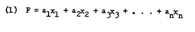
Linear combinations are derived by using several judgmental criteria or the analytical criterion of least squares principle. The latter suggests a close resemblance to regression. However, the peculiarity of factor analysis lies in the fact that a number of linear combinations each giving one factor is more common. In short, it is not at all unusual to obtain a small number of factors in any data analysis. Thus, we can more generally stat, as follows:

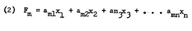
In factor analyzing a data matrix, two sets of values are obtained which are known as factor scores and factor loadings.4 A factor score is individual’s score as a result of linear combination of his manifest scores. Thus,

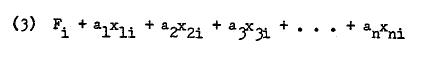
Since there are as many scores per individual i as there are linear combinations (factors), we may generalize (3) to this:

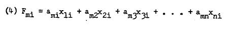
A factor loading is the correlation between factor scores and the manifest scores of the individuals in the sample. These correlations may be high or low, positive or negative, depending on the dependence of manifest variables and the particular method of factor analysis. We may describe a factor loading as

Factor analysis is more appropriately a set of data reduction techniques rather than a single unique method. Much of the confusion in marketing literature stems from not appreciating this fact. The set is created as a result of a variety of options available to the researcher for analyzing data. These options can be grouped as with regard to (1) nature of data matrix to be factored, (2) weights or coefficients to be specified in making the linear combinations, and (3) derivation of new (rotated) factors by transformation of original factors [49, 52].
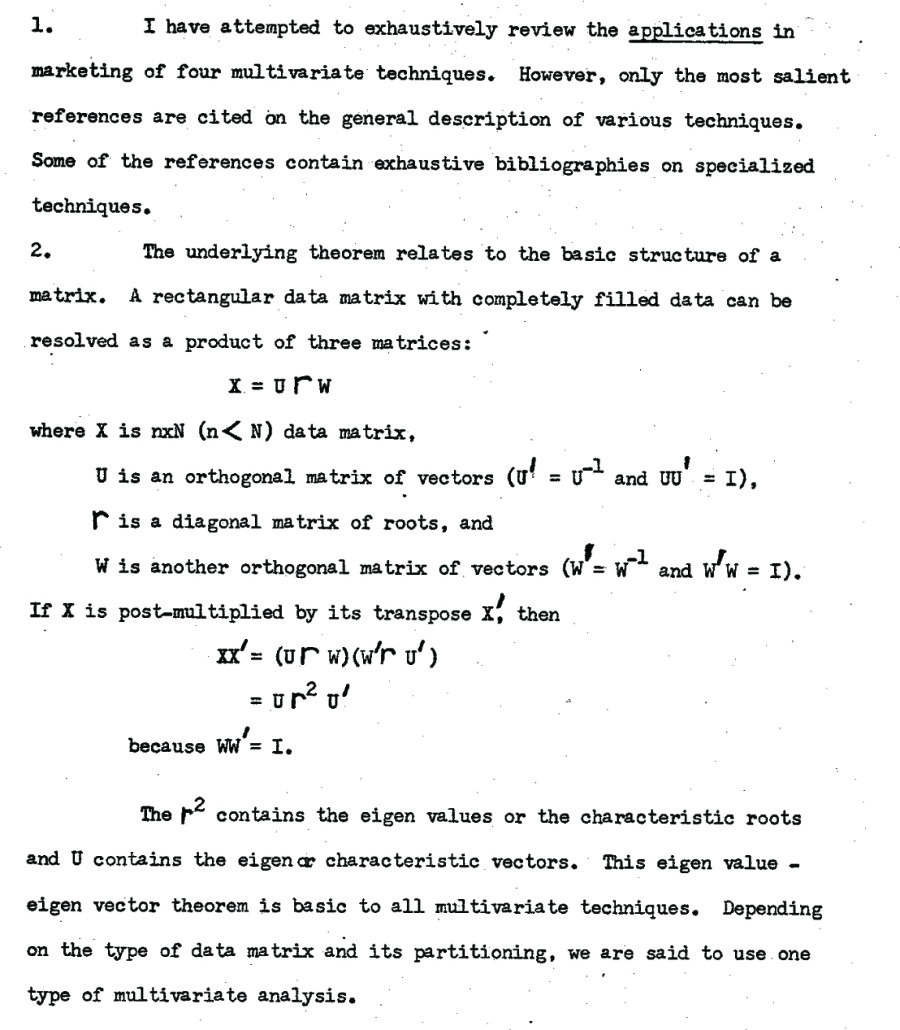
The option related to data matrix is with regard to factoring either a correlation matrix, a covariance matrix, or a cross—products matrix. Any multivariate analysis begins with a data matrix X consisting of n rows representing variables and N columns representing individuals. .n some cases, it is advantageous to redefine rows and columns by transposing the data matrix. The cell xji refers to i individual’ s response on jth variable. This data matrix contains three types of information: level, dispersion and shape of variables or individuals. In some analyses, ail the three types of information are relevant. In that case, we obtain a cross—products matrix XX by post—multiplying the data matrix with its transpose. Each cell element contains sums of squares or cross products. If only dispersion and shape are important, we may at first set levels of all variables equal, preferably at zero level, aid obtain transformed coil values which are deviation scores. A cross—products matrix of deviation scores becomes a covariance matrix when each cell is divided by the number of variables. Finally if both level aid dispersion are not relevant to the analysis we may equate both of these across the variables. One way is to obtain standard scores where, means are equal to zero and variances are ail equal to unity. The cross—products of a matrix of standard scores then results in the well-known and common correlation matrix.
Obviously, covariance and correlation matrices are one specific way of removing the effects of level and disperson on the data. They are commonly used because of their mathematical relationships to known distributions such as normal distribution. However, any other method of equalizing level aid dispersion would be relevant as data input for factor analysis. Of course, there are some situations where a particular type of data matrix is almost mandatory. For example, when the units of measurement of variables are quite diverse so as to lack common dimensionality, it is desired that data be standardized. On the other hand, if the researcher believes, based on his theory, that he should expect individual differences in the sample on level aid dispersion, it is better to use the cross—products matrix [92,95].

Finally, there are six separate ways that data can be correlated with the use of cross—products, covariance or correlation procedures because, in general, we have three kinds of information:
variables, people, and separate time periods. Holding one dimension Constant, and using the second dimension as replications, a cross— products, covariance or correlation matrix can be obtained on the various elements of the third dimension. For example, we may get a variable—by-variable correlation matrix, or people—by-people correlation matrix or time-by-time correlation matrix. Cattell [13] has given various labels to the six types out of which factoring a variable by variable at a point in time correlation matrix is called K—type factor analysis, and that of a person—by—person correlation matrix at a point in time is called Q—type factor analysis.5
The second option is the choice of weights for making linear combinations. This option is two—fold; judgmental methods and analytical methods. As the name implies, judgmental procedures only approximate some exact solutions and there is no statistical rationale for their choice. The best known of these procedures are centroid method, bifactor method and multiple group method. Among the analytical procedures which use the basic structure theorems of matrix algebra, the most widely known is the principal components analysis. Finally, both the judgmental awl analytical procedures give further options (particularly in a correlation matrix input) s to the diagonal values.6 The reader is referred to Harman [49] and Horst [52] for detailed description on this aspect.

The third option is regarding the derivation of new (rotated) factors by linear transformation procedures. Once again, there are two broad types: judgmental or analytical. The judgmental procedures all date back to Thurstone’s simple structure principle whereby a factor is rotated to an extent that any one variable is highly loaded on one and only one factor. The analytical procedures use a number of variations of this simple structure principle. The two most common analytical procedures are quartimax and varimax rotations. The third option is resorted to by researchers for better interpretation of the results, and has no statistical significance per so. It is also the most controversial aspect of factor analysis. Once again, the reader is referred to Harman [49] and Horst [52].

It is obvious that possible combinations of the three types of options and further suboptions in each type generate hundreds of separate factor analyses.

Applications in Marketing

It is no wonder that despite widespread knowledge and diffusion of factor analysis in marketing, there exists considerable confusion and heterogeneity of opinions among marketing scients [19, 28, 29, 42, 60, 76, 90, 118]. We will review the applications of factor analysis in marketing by looking at five separate uses to which the technique has been put.

(1) The first use is to infer the dimensions which latently order products or brands in terms of preference. Data are obtained on the ranking or rating of products in terms of overall preference or liking. Then after factor analyzing them, the researcher looks for clues outside the data to interpret and name the factors. The factors are, therefore, loaded with surplus meaning which adds subjectivity to the analysis.

A good example of this type of analysis comes from Stoetzel [109]. Be obtained three factors based on ranking of various types of liquors (Scotch, gin, Champaign, etc.) by a sample of French consumers. After looking at the factor loadings, he labeled them as sweetness, price and regional popularity factors based on his external knowledge about the liquor industry.7 Similar studies have been done on preferences for Chesire Cheeses [50], for foods [89], for television shows and magazines [.25, 26, 69, 110, 119], and for brands of durable appliances [101]. The latter study reveals a good deal of brand generalization across several product classes for brands such as General Electric, Sears, Westinghouse, Hotpoint and Frigidaire.

The problem in these studies is of course, attributing causality to the underlying traits which are at best inferred from the researcher’s own knowledge of the market outside the data. The advantages are that it is simple, assumes no knowledge on the part of the researcher, and some— tines reveals unusual things about the phenomenon under investigation.

(2) The second use of factor analysis is to obtain structure among a set of attributes related to a product. The researcher has sufficient knowledge about the product to identify its characteristics. The interest is to see which of these characteristics go together and whether they could be meaningful in terms of overall preference for example, collected data on a large number of scales related to coffee attributes and reduced them to a few factors which seem the underlying determinants of buyer’s preference for coffee. Unlike the first use, the interpretation and labeling is limited to the data itself. Other studies of include obtaining terms of attributes related to corporate character [2?], to supermarket choice [32], to propensity to buy [93] to best selling books [51], and to brand choice [3]. Special mention must be made of factor analysis of semantic differentials to obtain corporate image [18].

An interesting study by Lunn [73] attempted to establish correlates of overall preference for a brand in terms of specific brand characteristics. Sheth and Ring [102], on the same lines, find that out of several evaluative characteristics of a brand, only a few load on the same factor with the overall evaluative preference scale. This suggests that consumers prefer that brand on a very few attributes. This seems to hold for several brands in three separate product classes.

(3) The third use of factor analysis in marketing is to cluster variables or individuals for classification and segmentation. To classify variables the R-type factor analysis is done whereas to classify Individuals, the Q—type factor analysis is done.8 Only a handful of studies in marketing have used factor analysis for this purpose. By far the best is that of Stephenson [108] on image of public utilities based on his Q—sort technique [107]. Similarly, Clevenger Lazier and Clark [18] compare corporate images of a tobacco and an appliance company from two independent samples. They find good congruence between the two concepts and between the two samples. Finally, barban and Grunbaum [4] classified 10 advertising stimuli on a set of semantic differentials, and found considerable differences between white and negro respondents, I am somewhat surprised to find no use of factor analysis in the areas of pilot testing and motivation research where Q-type factor analysis seems so relevant.

(4) The fourth use of factor analysis is to isolate, based on factor analysis of data, those variables which show greatest promise for further analysis. For example, Twedt [117] isolated three variables based on a factor analysis of 19 predictor variables (various aspects of advertisements such as size, color, layout, etc.) and the criterion variable of readership. Then he used these three variable as predictors of readership by- doing multiple regression arid obtained a correlation coefficient of .76 which is very high, to say to least. The only other study is by Sethi 1.95] to isolate -.ore salient socioeconomic variables.

(5) Finally, factor analysis is used to obtain factor scores of individuals in the sample for further analysis. Not only does this conversion of manifest scores to factor scores reduce large se of data to a more manageable level, it also removes co linearity in the original variables. Messy [74, 75] has dome the pioneering work in this direction.

Others include Farley [33] to explain variability in brand loyalty across products; Green, Frank and Robinson [46] to cluster potential test market cities; and Campbell (12] to use factor scores derived from socioeconomic variables to do step—wise regression of the size of the evoked set.
Although factor scores have been mostly used for further regression or discriminatory analysis (in fact, the motivation to factor analyze the data is to remove. co linearity which is otherwise a problem in regression), it is possible to use any other statistical technique on them, such as parametric or nonparametric tests of hypotheses about means and variances [97].

New Directions

There are several major extensions of factor analysis in analyzing marketing data. I will point out two that seem most relevant arid on which some research is already done.
(a) The first extension is to use factor analysis on classificatory data – dichotic, tracheotomies, etc. A large number of variables in marketing are classificatory which makes this extension very useful aid relevant. Use of factor analysis on classificatory data vas first suggested by Burt [10] and Guttman [48] independently. Burt’s approach seems more useful because of its close resemblance to Chi squared analysis of manifold contingency tables.

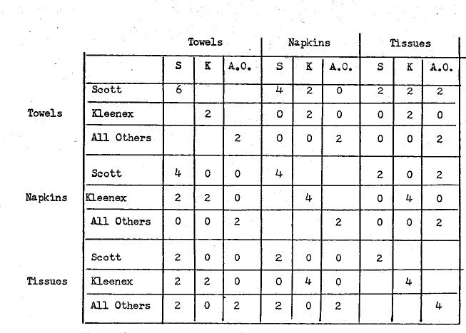
Let me illustrate this with an example [99]. Suppose we have information from a sample of consumers as to which is their most preferred brand in several product categories. Further, suppose that our interest is in knowing the extent of brand generalization among three paper products, namely towels, napkins and tissues. The following table shows the reactions of 10 consumers to various brands of paper products classified as Scott, Kleenex and All Others.

In the above table, 1 represents the most preferred brand and represents less preferred brands. It is obvious that in a given product category, a buyer can have only one brand as the most preferred brand. The brands are, therefore mutually exclusive and exhaustive within a product class.
Looking at the data, it is evident that the first two buyers all loyal to Scott brand and manifest complete brand generalization. Similarly, fifth and sixth buyers are loyal to Kleenex. The last two buyers are not loyal either of these two brands but could be loyal to some other brand which is part of All Others. Now if there wore complete loyalty and generalization to the three categories of bran, we must obtain perfect correlation across product classes. Furthermore, since there are three mutually exclusive and exhaustive categories, we can find extent of generalization f or each category. In other words, for a compete generalization, there will be only three factors. On the other hand, if there is no consistent preference at all across two or more product classes for any one category variable will be unique and hence we will have nine factors. In between any other number of factors will be obtained depending upon the extent of brand generalization for each of the brands.

The first step is to post-multiply the data matrix by its transpose to obtain a cross—products matrix. The following table gives the cross-products matrix. It will be noted that it is a square symmetric matrix and is a type of manifold contingency table. Also, it is a super- matrix in which the diagonal matrices have elements only in the diagonals. Looking at the appear that we should expect about five complete generalization among a the three brand categories, and the last two representing the divided loyalty between two brands such as Scott Towel and Kleenex Napkins and Scott Towel and All Others Tissues.

Just as we can understand brand generalization, we can also understand brand switching over time within the same product class. Each time period in place of each product class will now be a class factory variable. My preliminary study on brand switching over time shows two cross—products matrix, it would factors: the first three r.pr.— subset of consumers for each of things. First, that brand loyalty a number of brands can be measured for every consumer. In other words, brand loyalty is multi… dimensional in the sense that a consumer can be loyal to more than one brand (with differential degree of loyalty). Second, it is possible to arrive at measures of aggregate market shares of brands for the total time period studied in which such market share is a function of both the frequency of purchase and pattern of brand switching. In other words, market share is weighted by consumer’s extent of loyalty which seems a more suitable measure at least for managerial evaluation.

(b) Another major extension of factor analysis is to use it for obtaining functional relationships among the manifest variables [100]. The essential idea is that in a time-series data (such as purchase frequency for various months of a year by a sample of households), each cell entry xii (for example, i individual’s purchase frequency at the time-period) can be considered a point on a curve where the independent axis is some unit of time and the dependent axis is the particular phenomenon under investigation with which the cell values are filled. In other words,

The aim (factor loadings in the normal sense) represent aggregate parameters and (factor scores) represent each individual’s for his functional relationship. Using this approach, it i possible to do curve fitting for all linear and several nonlinear functions. The parameters meet the least squares criterion. The technique, however, has several advantages over curve fitting. First, it gives parameters for each individual consumer, in addition to aggregate parameters. Second, several types of curves, each varying in shape for different individuals, can be estimated in one analysis. Third, a very few column vectors (two to three) summarize a large variety of individual parameters based on which we can classify individuals as belonging to particular functional relationships.

I have used the functional approach to obtain brand loyalty scores of individual consumers based on their frequency and pattern of purchases over a discrete time-period r98). Obviously, in time-dependent sequences, pattern makes the difference between two individuals who have the same frequency of purchase.

Profile and Cluster Analysis

A second major multivariate technique is profile or cluster analysis. Profile analysis is a generic term for all methods concerning grouping of individuals. Cluster analysis is a generic term for all methods concerning grouping of variables. The procedures for both cluster and profile analysis are very similar, and hence we will refer to both of them as profile analysis.

Profile analysis involves at least two separate steps. The first is the, measurement of similarity between two persons or variables. The second is classification of persons or variables based on the similarity measures. A series of cut—and-try methods have been proposed to perform profile analysis [2, 22, 85, 86, 103, 104]. Most of these calculate distance between two persons by putting them in some sort of space. In general, a person with his scores cm n variables is considered a point in n-dimensional space. The distance between two points gives a measure of similarity: the greater the distance the less similar the two points. Then several arbitrary methods are available which specify the cut-off point for the marginal person to be included in a group (103, 104).

The two most common distance measures are calculation of absolute differences and distances based on Pythagorean Theorem. Mathematically, they can be stated as:

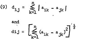
where i and j are two persons or points in n-dimensional space constructed from measurement on k scales.

The similarity measure d. in the above methods contains all the three types of information: level, dispersion and shape. By removing one or more of these, several other distance measures are possible.

Recently, Sokal and Sneath [104] have suggested several procedures for classification under the name of numerical taxonomy. For an excellent description and review of these, see Frank and Green [36].

Most of the profile analyses suffer from two problems. First is the lack of invariance of similarity between two persons resulting from adding or dropping the dimensions on which they are measured. This becomes a serious issue when the dimensions for comparison are based on convenience and, at best, judgment instead of any theory. The second and related problem is the dimensions. If the dimensions are not orthogonal, the distances based on space become less meaningful.

Applications in Marketing

Except for the graphic representation of semantic differential scores (79) as profiles, the application of profile analysis is very recent in marketing. The first attempts relate to measurement of similarity between self—concept and some consumer behavior variable where attempt is made to show greater congruence between the two [6, 47]. However, classification of consumers in these studies is already known based on the particular consumer behavior under investigation. The pioneering efforts to measure similarity and then classify objects or people from Green, Frank and Robinson (46]. They used the distances to obtain clusters of cities which are potential for test marketing. A good review on classification procedures recently appeared in Applied Statistics [61].

The only other research analysis in this area comes from Myers and Nicosia [83) based on Tryon’s conceptual and computerized methods of cluster analysis [113, 114. 115].

New Directions

Despite the simplicity, profile analysis is not extensively used in marketing. It does seem potentially relevant in several areas of marketing outside consumer behavior per se. For example, Railing law of retail gravitation can be more accurately represented in today’s economy by taking a set of forces (brand choices in the store, pricing. parking convenience, checkout counter facilities, convenience and ease of in—store shopping, cleanliness of the store, etc.) on which the stores can be compared in terms of similarity. From this, we can obtain clustering of stores in a specific region. Another example is the evaluation and promotion of brands based on their similarity at the market place. For example, a company such as General Foods may cluster various types of frozen juices based on the evaluative judgments of the consumer and the retailer.
Profile analysis, however, doe, not lend itself to algebra, and hence analytical solutions. On the other hand, due to the level of maturity of the discipline, analytical solutions are more desirable. There are two directions in which some of the arbitrariness in profile analysis can he eliminated. First, it is possible to factor analyze a similarity matrix D obtained from the various values. The factors will then cluster individuals on analytical grounds [57, Chapter 6]. Second it is possible to combine both the steps in profile analysis, and obtain an analytical solution if we factor analyze a cross-products matrix of individuals.

Discriminatory Analysis

Discriminant analysis is useful in situations where total sample is divided into known groups based on some classificatory variable (sex), and the researcher is interested in understanding group differences or in predicting correct belonging to a group of a new sample based on the information on a set of predictor variables.

Discriminant analysis, therefore, can be considered either a type of profile analysis or a type of multiple regression. As a profile analysis, its significance lies in the structure of weights obtained which discriminate various groups. Then, it is sometimes referred to as structural analysis [68]. As a multiple regression, its significance lies in providing predictive power to the researcher in terms of classifying individuals more accurately than by chance. In either case, the criterion variable is Single and classificatory.

Discriminant analysis entails transformation of scores of individuals on a set of predictor variables by using a set of linear weights. The transformed value is called the discriminant score. This score is treated as projection of a point, on the discriminant axes and depending on whether it lies above or below the discriminant line, the individual is classified as belonging to one or the other group. The linear transformation of raw scores into discriminant scores can be represented as:

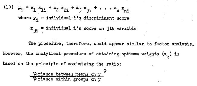
This is analogous to one—may classification in analysis of variance [34].

It is possible to obtain more than one discriminant axis similar to factor analysis. However, the total number of axes do not exceed the number of groups minus one. In a two—group situation, therefore, only one discriminant axis and one discrirninant score for each individual are obtained.

Once the discriminant axis is obtained, the function could be tested for significance. Then based on the discriminant scores, individuals in the sample void be classified in one of the groups. The proportion of correct classification then is compared against what could have been predicted by chance without any knowledge of the scores on the predictor variables. To this extent, it resembles the Bayesian approach.

It is, however, more appropriate to validate the analysis by using the discriminant weights on another sample of individuals because predicting on the same sample from which coefficients are derived is shown to result in biases [39].

Applications in Marketing

A large number of research studies in marketing have recently applied discriminant analysis mostly for prediction purposes. Evans [30], for example, attempted to discriminate new Ford and Chevrolet buyers based on personality needs, socioeconomic variables, and a combination of both with little success. Recently, however, Ito [58] successfully discriminated loyal and switching Ford and Chevrolet buyers on the basis of nine attitude scales. However, he used intention measures for the second purchase as opposed to actual purchases. A number of studies [23, 37, 38, 64, 65, 66, 67, 88, 91] deal with prediction of innovators from non— adaptors or late adopters on a series of socioeconomic, personality, psychological and purchase characteristics. The success is only moderate. Other areas of applications include discrininating among listeners who sent f or a program guide from those who did not [77], among various types of holders of savings accounts [17], among consumer decision types on personality variables [8], among social classes [41], among those who intend to buy [87], and to obtain scale values in an advertising study [5]. Perhaps the most extensive use of discriminant analysis in a single study comes from Sethi [95] who attempted to discriminate high and low buyers of brands of analgesic on socioeconomic purchase characteristics and a combination of both types of variables.

In using discriminant analysis for prediction purposes, there are two problems which a researcher generally encounters. First, the dependent classificatory variable is more often then not forced on the data by the researcher with the result that there exists an overlap between groups to an extent that separation of groups is not powerful.

A greater caution is needed among the users of discriminant analysis in their definition of classificatory dependent variable (68, 97). The second problem concerns validation of the analysis pointed out earlier. If the same sample is used .it overe8timates the predictive power of the discriminant function (39). A pragmatic suggestion is to split the sample into half, using one half for analysis and the other half for validation.

The above-mentioned problems have led King (68) to suggest that we may use discriminant analysis not so much for prediction as for relative importance of predictor variables based on structural analysis of discriminant coefficients.

New Directions

With sufficient care a number of exciting applications of discriminant analysis can be made in marketing. I have, for example, suggested that various marketing strategies may be considered ‘experiments,’ which could be evaluated on a series of performance measures. Each experiment would be a group, and performance measures would be various predictor variables. Similarly, various advertising campaigns can be treated as experiments and then evaluated. Not only this will show the relative effectiveness of various strategies, it will also show the relative effects on various performance measures (97).

Another important new direction is the extension of discriminant analysis in situations where the predictor variables are also classificatory (only binary though). See Clarigbold [16] for a good description of this. This extension is quite useful in view of the fact that a large number of variables such as sex, religion, occupation, etc. are classificatory. It is somewhat surprising that Fisher (34) himself suggested such extension and still it is not widely known in marketing [59].

Canonical Analysis

Canonical analysis is an extension of multiple regression to a situation where there are more than one criterion variables. There are, then, two sets of measurements one criterion set and the other predictor set, which have to be correlated. The underlying principle is to create a linear combination of each set of variables for each individual by obtaining a set of weights which maximize the correlation between the two sets.

Canonical analysis is appropriate when the researcher is more interested in the overall relation between the predictor and the criterion sets. He may then isolate those predictor variables which contribute most to this overall relation. In addition, he may also note which of the criterion variables are more affected.

Applications and New Directions in Marketing

Canonical analysis is scarcely known to marketing researchers. Otherwise, there are so many areas of consumer research, advertising research and product research where it is most appropriate but no study seems to exist. I hope the recent summary of the technique by Green, Halbert and Robinson [45] will enable marketing researchers to more fully appreciate the technique. The only study in which its use was made is by Kernan (63). He obtained an overall relation between a set of choice decision behaviors and a set of personality variables.

In consumer behavior, most of the variables of interest to the marketing practitioners have multi-attributes. For example, brand loyalty is indicated by probability of purchase, time interval between purchases and magnitude of buying. Consumer’s liking of a brand is likely to be based on a number of brand attributes. Thus when we want to measure effectiveness of a set of controllable variables, canonical analysis is obviously relevant since effects are numerous.

There are two possible extensions of the technique which may prove useful in marketing. The first is to perform canonical analysis on a cross—products matrix similar to factor analysis. Since the input data matrix retains information on level and dispersion, it may prove more appropriate when we know that individual variability is likely to be high. The second suggestion is to extend the technique to binary data.

Summary Statement

Above I have attempted to review multivariate analysis of marketing data. I have hinted several possible extensions of the techniques. My own exposure to, and involvement in, multivariate techniques has convinced me that they are extremely useful in marketing. With the availability of canned computer programs, it seems inevitable that the techniques will diffuse in marketing research.

Foot Notes

References