A. Marvin Roscoe, Jr., American Telephone & Telegraph Company and Jagdish N. Sheth, University of Illinois
The objective of the study was to explore the appropriateness of several statistical techniques in developing predictive models of consumers’ long distance telephone expenditure based on the analysis of socioeconomic and demographic characteristics. Specifically, the paper examines the relative efficacy of stepwise multiple regression, monotonic AID (Automatic Interaction Detector) and free AID in analyzing large scale data.
Description Of MRIS Data Bank
Most consumer behavior research to date has been ad hoc, fragmentary, and exploratory. Only recently have large corporations begun to generate continuous and systematic information about the market place as part of their marketing information systems. The Bell System Companies provide communication services in the 48 continental states and the District of Columbia to 104 million telephones, 83% Or the total telephones in the United States. The need to understand this enormous market is self-evident, not only from a traditional marketing view but also from the social and economic considerations inherent in the management of a regulated utility. To help meet this need, a large scale Market Research Information System (MRIS) has been established, consisting of a national longitudinal panel of some 60,000 customers representing both the business and residence markets.
MRIS panel members were selected by multistage stratified sampling procedures from the customer files of each of the one hundred accounting offices of the Bell System where customer billing is performed. A panel of 600 customers, evenly divided between business and residence customers, was selected from each Of these accounting offices. Currently, the MRIS data bank contains more than 126 million card image record, and is growing at the rate of 3 1/2 million record each month. The MRIS panel excludes certain types of accounts, such as the U.S. Government, which are handled separately from a communications view point, and certain specialized types of communications services such as private line and data services.
For each panel member, the MRIS data bank stores the following information:
1. A basic equipment record consisting of service and equipment data, such as the number and type of telephone lines, number of extension phones and other vertical (optional) services including Princess* and Trimline* phones, Touch-Tone* service and additional Directory listings. These data are updated whenever panel members change their service or equipment. *Registered trademark of the Bell System.
2. A billing amount record listing charges for local service, additional message units (where applicable), a summary of long distance billing, taxes and other charges or credits as shown on the customer’s bill. This record $s expanded every month.
3. A long distance record listing billing details for each message found on the customer’s billing statement, such as the date and time of the call, type of call (direct dial or operator handled), length Of conversation and amount of charge. This record is also expanded each month.
4. A demographic record containing a socioeconomic and demographic profile of the residence customer’s household unit. These data have been obtained from a m*il questionnaire, and include age, sex, education and occupation of the head of household, family size and composition, its mobility characteristics and family income. The residence profile is updated every three years, and consideration is presently being given to collecting additional information on the residence customer’s fundamental value system as well as his generalized attitudes toward the telephone as a means of communication.
To be able to comprehend this enormous amount of information at the microlevel of the individual customer, basic research is underway to develop analytic strategies in the interest of building predictive micro and macro models of buyer behavior for the telephone industry.
This paper represents one Of our proJects designed to develop an understanding of the long distance telephone behavior of the residence customer. The relationship of socioeconomic and demographic factors to long distance behavior is especially important to insure that the rate structures filed by the Telephone Companies and approved by the regulatory agencies are equitable to the various socioeconomic customer segments in the country [The authors are well aware of the controversy with regard to the usefulness of demographic factors in predicting consumer behavior (Yankelovich, 1964; Frank, 1968; Bass, Tigert, & Londale, 1968). However, given the regulated nature of the utility industry, it is necessary to understand and to be able to predict the impact of corporate strategies on different socioeconomic segments of the population.].
In order to examine the characteristics of the data and the associated problems in their analysis, the study was limited to the 793 panel customers from two Northeastern states. The two groups of customers were chosen on the basis of comparability of long distance expenditure, providing a sample size that would not unduly favor one particular analytic technique. The focus of this paper is, however, data analysis and not inference, although decision and predictive models are being built based on the findings from this type of data analysis utilizing larger and more generalized samples Of the population.
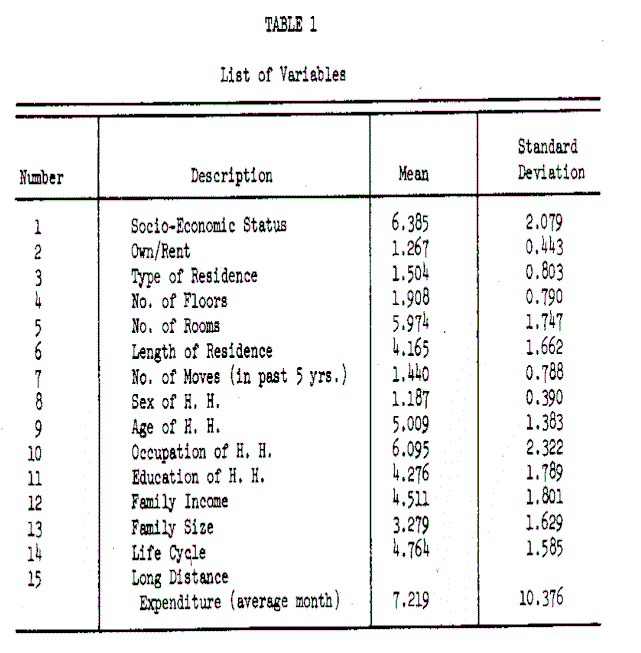
Table 1 lists the fourteen socioeconomic and demographic variables and the dependent variable, long distance expenditure [The term expenditure properly connotes the aspects of consumer buying behavior. Increasing the consumer’s level of long distance expenditure is a very important consideration to the telephone industry. Since the distribution channel is always available and there are frequent periods of available capacity, increased calling during these periods can have very obvious economic implications to society.], with their means and standard deviations. To avoid the effects of seasonality and holidays, the long distance behavior variable was based on the monthly average of a year’s history for each residence customer, expressed in dollars and cents. The dollar signs have been omitted for the sake Of simplicity. Among the fourteen socioeconomic and demographic variables, two index variables have been included, the socioeconomic status (SES) index and the Life Cycle index. The SES index is a score developed from a composite of the education and occupation Of the head Of household and family income level using the procedures Of the U.S. Bureau Of the Census (1963). The Life Cycle index is determined from the age and marital status of the head of household and family composition, following the procedures used by the Survey Research Center at the University of Michigan (Lansing & Kish, 1957).
Problems Of Data Analysis And Alternative Statistical Approaches
In Figure 1, long distance expenditure is plotted for each socioeconomic and demographic variable. The variables have been grouped in four categories derived from a prior factor analysis of these data. Examining the plots clearly points out the following data problems typical of most survey research (Morgan & Sonquist, 1963; Carman, 1967 9 Sonquist, 1970):
1. All of the demographic variables are discrete rather than continuous, although many of them do have successive class intervals containing large numbers of observations.
2. The variables have a mixture of scales consisting of nominal and interval-scaled data.
3. The relationship of long distance expenditure with many of the demographic variables is not linear.
4. In some cases, the relationship is not even monotonic.
5. The demographic variables may be related to long distance telephone behavior in an interactive manner rather than in a simple additive manner.
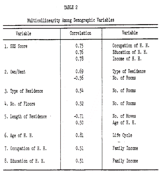
6. The demographic variables tend to be correlated with one another, which may be a serious problem when using regression analysis (Blalock, 1963) . Table 2 summarizes some of the highly multicollinear variables.
Starting with a large body of empirical data and little or no prior theory with which to develop functional relationships, it is difficult to construct a multivariate model without first investigating the effects of these data problems as they relate to analysis by standard statistical methods. In fact, the authors believe that the blind use of a statistical method may produce great harm from misinterpretation of the data, and could even result in throwing out important data as irrelevant or useless for a marketing problem.
Our objective was, therefore, to first explore several analytic strategies which take into consideration, to varying degrees, these data problems. Stepwise multiple regression, AID with the monotonic restriction on the predictor variables, and AID without the monotonic restriction were chosen as the three alternative strategies because each responds somewhat differently to these data characteristics. Such a combination should, therefore, both avoid the problem of forming an unsupportable advance hypothesis and give the analyst perspective on the actual structure under observation.
Multiple regression is a robust method, rich in both data analysis and inference. In addition, regression analysis, with some variations, can take into account the problem of mixed scales and class interval data. For example, by using dummy variables it is possible to include a number of nominally scaled demographic descriptors such as ownership of residence and sex of the head of household. Finally, stepwise multiple regression considers the problem of multicollinearity by developing partial correlations at each step, thereby eliminating variables that are highly correlated with variables already included in the regression equation. [There are several other methods for handling the multicollinearity problem, such as examination of the simple correlations or factor structure of the correlation matrix. In fact, due to the order bias built into stepwise regression, other methods should be used to reduce the collinearity problem.] However, since the regression equation is a linear additive model, it is not capable of effectively handling the problems of nonlinear, nonmonotonic and interactive relationships. [Regression theory can handle nonlinear and interactive relationships, but these need to be developed a priori based on some theory of Judgment. Without theory to suggest rational approaches, the number of nonlinear transformations and the combination of interactions are too many for regression analysis to solve efficiently.]
The objective in AID analysis is to partition the total sample into an optimal set of nonoverlapping subgroups, developed from the profiles of the predictor variables, whose categories explain more of the variation in the dependent variable than do any other set of subgroups. This objective is achieved by a sequential partitioning of the total sample into two subgroups based on the split of a single predictor variable which produces the largest ratio of between sum of squares to total sum of squares. This process is repeated on each of the subgroups until some minimum level of explained variance is encountered or a minimum sample size is reached in the subgroup. Thus, one-way analysis of variance is explicitly included in the analysis.
Because the splitting of groups is sequential, the AID analysis is a stepwise procedure similar to the stepwise regression method, and so minimizes the problem of multicollinearity. However, the optimal split at each step is not based on a predictor’s contribution to reducing the error variance in the total sample but the variance in the subgroup.
Several researchers have used the AID technique in marketing, either for developing segments (Assael, 1970) or for model building (Carman, 1967; Armstrong & Andress, 1970). The technique itself is described by Morgan and Sonquist (1963), Sonquist and Morgan (1964), and Sonquist (1970). The AID program is capable of handling both the categorical and class interval predictor variables, regardless of whether their relationship is linear, nonlinear or nonmonotonic with respect to the criterion variable. Of course, the criterion, or dependent, variable may be continuous and in the case of long distance expenditure it is. Finally, and most importantly, this procedure is capable of handling both the additive and the interactive relationships of a set of predictors with the criterion variable.
Two types of AID analyses were used to separately examine the nonmonotonic and the interactive effects of the relationships between long distance expenditure and the demographic variables. The first, monotonic AID analysis, preserves the ordinality of the predictor variable when it is chosen as a candidate to split the sample. Therefore, the two new subgroups are defined as above and below the boundary of a category interval of the predictor variable. For example, given the eight categories of income, there are only seven (K-1) comparisons possible by splitting the group at each of the adjacent categories. By definition, therefore, monotonic AID analysis is capable of handling nonlinear relationships as long as they are monotonic or order-preserving.
The second procedure, free AID analysis, allows the split on a predictor variable without regard to the order of the categories of that variable. Thus, there is a much larger number of combinations of the predictor variable categories which may be examined to split the sample. This removes the nonlinear restriction and allows for the analysis of a nonmonotonic relationship if one exists between the predictor and the criterion variable.
Comparative Data Analysis And Results
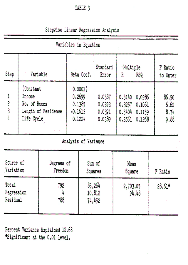
The stepwise linear regression analysis was performed using the UCLA Biomedical computer program BMD 02R (Dixon, 1971). To avoid highly collinear variables and random effects, an F value of 3.85, comparable to 0.05 level of significance, was set for a predictor variable to enter into the equation. The results of the stepwise regression analysis are summarized in Table 3. The multiple R was 0.36, resulting in 12.68 percent of the variance in long distance expenditure being explained by four of the demographic predictors. These four significant predictors and their associated explained variances are (1) family income, 9.86% (2) number of rooms, 0.75% (3) length of residence, 0 8% and (4) life cycle of the family 1.09%. The relationship is positive with income, number of rooms and life cycle, but negative with length of residence. In short, the greater the income, the more rooms in the residence unit, the later the stage of the life cycle, and the more recent the move of a residence customer, the greater the average long distance expenditure will be. It is interesting to note that life cycle as an index variable performed better than its component demographic variables but the SES index did not perform better than income.
Several questions are implicit in these findings. First, the bulk of the variance explained is concentrated in income (77.7%) with relatively little contribution from the other demographic variables. Secondly, the total amount of explained variance is relatively lower than might be expected [By setting a low F value (0.01) all of the 14 demographic variables were permitted to enter in the final step of the regression analysis. The predictive power increased to 14.25 percent. These results were replicated using the UCLA BMD 03R Multiple Regression Program. Unfortunately, the additional explanatory power has the inherent problems of instability and multicollinearity.]. And third, most other demographic variables fail to exhibit any relationship on a partial correlation basis. There are obviously two answers. First, no relationship may exist with these other variables, so that long distance expenditure is determined by other factors not in the equation. However, and secondly, it is possible that the linear additive model built into the regression suppresses any nonlinear or interactive relationship between the demographic variables and long distance telephone behavior. Unless the latter explanation is ruled out, good data may be discarded due to inappropriate analytic methods.
The monotonic AID analysis was the second method used. This procedure allows for monotonic, nonlinear and interactive relationships between the predictor variables and the criterion variable as noted. To avoid unstable results and to meet sampling error requirements, the AID analysis was based on the additional constraints of a minimum sample size of 30 in each final subgroup, and a minimum percent variance explained equal to or greater than o.6 percent at each step.
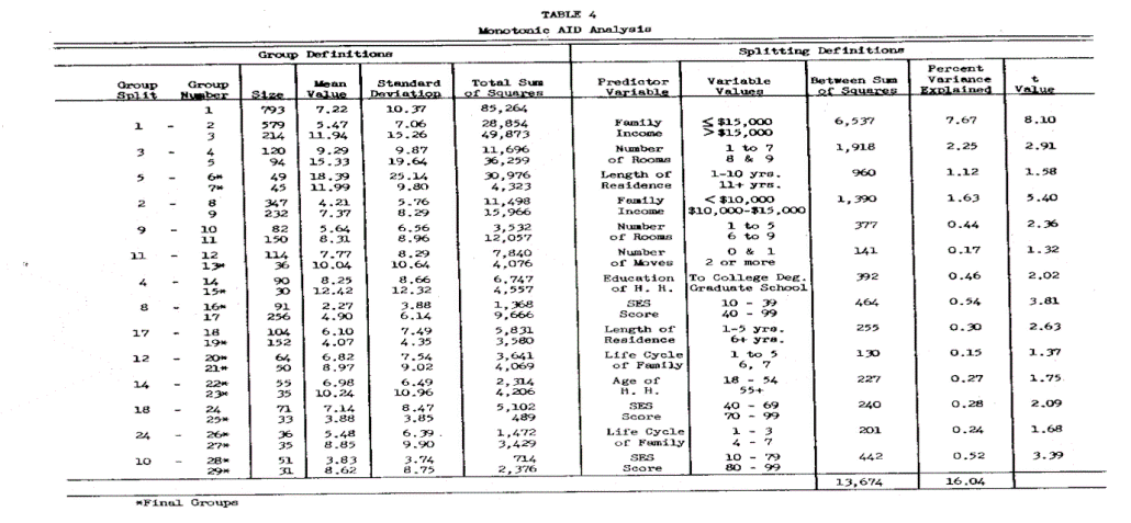
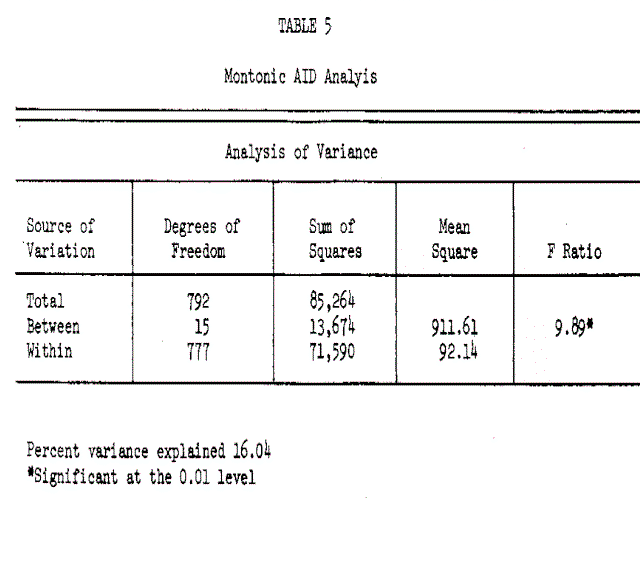
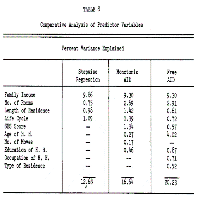
The statistical results are summarized in Tables 4 and 5. The explained variance was increased from 12.68 percent, using regression analysis, to 16.04 percent using AID and allowing monotonic and interactive relationships. Table 4 shows that the SES score, the education and age of the head of household and number of moves have entered into the analysis. The additional explanatory power comes from (1) the inclusion of these variables and (2 ) the increases in the predictive power of the variables as against the regression equation. The best examples of increased predictive power are the SES score, which was 1.34%, and the number of rooms which increased from 0.75% to 2.69% variance explained. These values are the summation of individual percent variance explained in Table 4. This increased predictive power can be explained by the fact that both of these variables have a step function with the long distance expenditure as seen from the plots in Figure 1. A similar step function in length of residence also slightly increases its predictive power.
On the other hand, the predictive power of income and life cycle decreased slightly in monotonic AID. This is largely due to the small number of cases at the upper end of the income scale and at the lower end of the life cycle index. These small cell sizes do not permit further subdivision due to the restriction of the minimum size in the final groups formed.
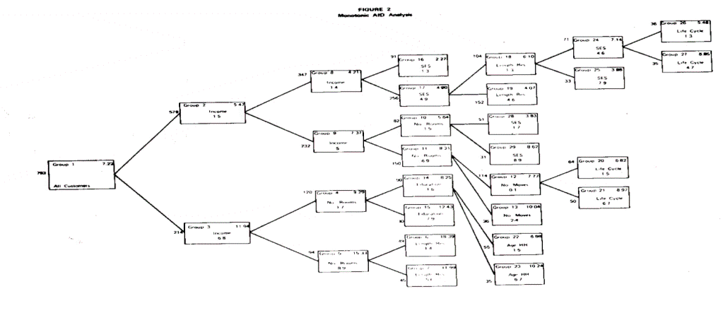
A careful examination of the group splits which result in large between sum of squares reveals that they are directly a function of the truncation in the monotonic relationship of the predictor variable with the criterion variable. Thus, the greater the rise of the step in the function between the predictor and the criterion variable, the greater the relative predictive power that variable possesses. Surprisingly, the interaction among the significant demographic variables is not as great as expected. This is shown in the tree diagram of Figure 2 by the relatively good symmetry of splits where the predictive variables appear on both branches of the split. Stronger interaction between the demographic and the socioeconomic variables had been anticiPated; however, this interaction does not seem to be Present in the data.
Finally, a very important benefit of monotonic AID analysis comes from the fact that it matches the managerial problem definition and decision-making process. Typically, marketing management is interested in market differentiation and discrimination for better marketing effectiveness. Furthermore, the market differentiation is based on segmenting customers who are presumed to have different wants and desires. The demographic variables are considered the most common casual factors in bringing these differences to light, especially by the regulatory and other governmental agencies in the utility industry. The AID results have been represented as a diagram in Figure 2 which is both meaningful and communicable to management. For example, it indicates that customers with income above $15,000, with residence units consisting of eight or more rooms, and with less than ten years of residence at their present location have the highest average of long distance calling and expenditure (group six). On the other hand, customers with less than $10,000 income and an extremely low SES score manifest the lowest amount of average monthly expenditure (group sixteen). Both of these extreme groups, as well as the other segments, are meaningful and relate to management’s prior experiences and decisions. In view of the fact that half the problem in successful marketing research is its effective communication, AID seems to be an advantageous analytical strategy.
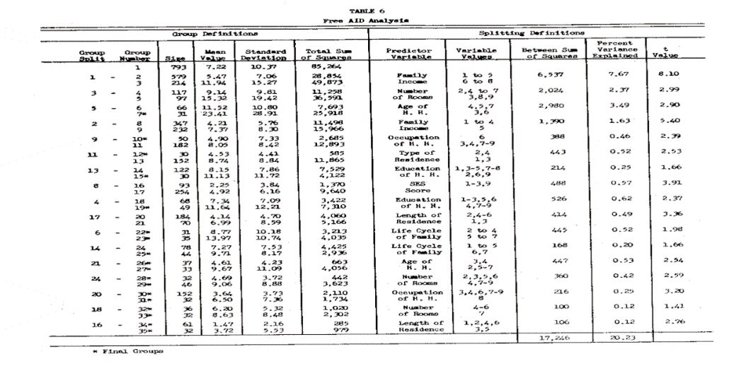
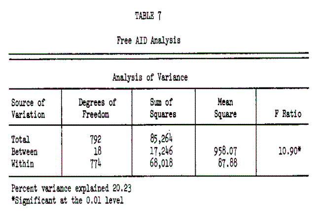
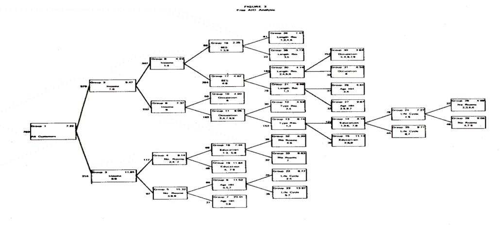
The third analytic technique is free AID analysis where the nonmonotonicity of the predictor-criterion relationship is taken into account in addition to the nonlinearity and interactive aspects. The same stopping criteria were utilized here (minimum subgroup size greater than or equal to 30 and o.6 percent variance explained at each step). The statistical results are summarized in Tables 6 and 7 and Figure 3.
Free AID analysis increases the predictive power of the demographic variables from 16.04 percent to 20.23 percent when compared to monotonic AID analysis. In the process, it includes occupation and type of residence variables; however, the bulk of the increased predictive power in this analysis comes from the demographic variable age of head of household, which has the greatest nonmonotonic relationship with long distance expenditure. Somewhat smaller increases in the predictive power of number of rooms, education, and life cycle are also due to their nonmonotonic relationship with long distance expenditure.
Surprisingly, the predictive power of both the SES index and length of residence decreased in the free AID analysis. This is attributable to the extreme skewness of the two predictor variables.
The free AID analysis reveals some subtle differences among customer segments which are hidden in the monotonic AID analysis. For example, the seventh group which has the highest average monthly bill, consists of customers who have greater than $15,000 income, both small and large residence units (three rooms and eight or more rooms) and who are both relatively young and relatively old (between 25 and 34 years and between 55 and 64 years). This was not fully revealed either in monotonic AID or in stepwise regression.
In view of the fact that the demographic variables which explain the variance in long distance expenditure differ for the three analytic methods, Table 8 has been prepared to summarize their relative contribution toward explaining variance in the criterion variable. Income, which was by far the best predictor, does not do as well in the AID analyses, primarily due to the problem of sample size in the extreme cells. The other three demographic variables – number of rooms, SES score and length of residence – did very well in monotonic AID due to two factors: (1) they have a step function relationship with the criterion variable, and (2) the distributions are badly skewed. Finally, age of head of household does best in free AID primarily due to its nonmonotonic relationship with the criterion variable.
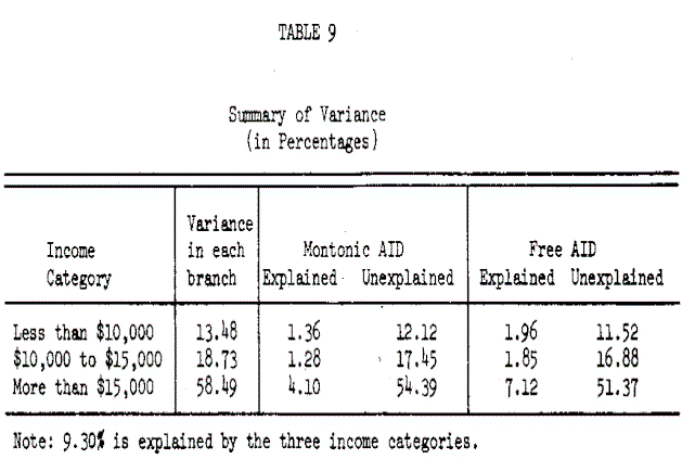
Having removed the nonlinear and nonmonotonic constraints and permitted interactive relationships in the analysis, the explained variance has increased from 12.68 to 20.32 percent. However, the unexplained variance still remains quite large. An additional advantage of the AID analysis is the ability to investigate the variance structure by customer segment. Monotonic AID and the Free AID analyses both developed three branches defined by low, medium and high income categories. These represent 44%, 29% and 27% of the sample size. Table 9 summarizes the effects for each branch.
Finally, noting that the bulk of the unexplained variance is in the high income branch a search of Table 4 and 6 shows that final group 6 in the monotonic AID analysis has 36+ percent of the total variance, and group 7 in free AID analysis has 30+ percent. These groups represent the tail of the skewed long distance expenditure distribution and should be evaluated further with a larger sample size in order to determine if the socioeconomic and demographic variables are capable of further explaining the variance in these customer segments. Until this is completed, an ultimate Judgement on the efficacy of these variables in explaining long distance expenditure can not be made. However, in the final analysis, it appears that approximately 30 percent of the variance can be explained by these predictor variables, which is in line with the initial expectations when the project was undertaken.
An Approach Toward Empirical Model Building
Comparing linear regression and AID analysis, it is difficult to say which technique is better. Each offers certain advantages that the other does not, and each has inherent problems. AID is much more flexible in data analysis and data handling because it requires the smallest set of assumptions. At the same time, it is extremely compatible with the managerial viewpoint of the market place. Therefore, it has the advantage of better communicating the market research results. Finally, the technique brings into bold relief the relationships among the variables, which leads the researcher to think of the interactive effects of a set of predictor variables. This is very likely to broaden his inductive theorizing process. On the other hand, AID is lacking in inferential capability. It is much easier to display the data than to build predictive empirical models with AID. This is because AID is largely based on analysis of variance principles and therefore requires prior experimental or matrix designs to enable any inferences to be drawn from the analysis. A second disadvantage with AID is less parsimony in data analysis and model building; considerable computation and search is inherent in the technique and the branching process often is fairly complex and lengthy, which reduces its usefulness from a pragmatic control standpoint. Finally, as was demonstrated in this paper, AID requires large sets of observations which must be fairly well-behaved in their distributions over the predictor and the criterion variables. In other words, skewness presents a serious problem in AID analysis.
Linear regression is very powerful in developing parametric models, and provides a mechanism for establishing point and interval estimates for predictive purposes. On the other hand, it presumes the data to be linear, error free and additively related to the criterion variable.
In view of the fact that in a regulated industry there is a need to build powerful predictive models, a systematic approach is necessary to develop inductive models of telephone behavior based on large scale empirical data. The data analysis reported in this paper, together with the following procedural steps are recommended for inductive model building. [The procedure is somewhat different from the two-stage AID-MCA linkage suggested by Sonquist (1970).]
1. Given a large scale data base, perform an initial AID analysis with as many predictor variables as are available or can be handled by the computer. The AID analysis will bring into bold relief the nature of the relationships among the variables resulting from a minimum set of restrictions with respect to the sample size of subgroups, split reducibility criterion and the priority ordering and coding aspects of the predictor variables. In short, a free AID analysis is recommended in this initial phase.
2. From the initial AID analysis, predictor variables should be selected for future analysis based on their explanatory power. The predictor variables should then be factor analyzed to estimate the degree of intercorrelations among them.
3. Choose a set of orthogonal predictor variables from the factor analysis results selecting the variable with the highest factor loading. The problems of error in measurement should also, be considered. For example it will generally be more advantageous to choose the age of the husband rather than the wife if both are loaded equally on a factor because of the possibility of response error in the latter variable. Similarly, education would be preferred over income. At the same time, the researcher must watch for the possibility of creating an index variable, especially when several predictor variables contribute to an equal, but smaller, extent toward the eigenvalue of the factor. Such an index, by definition, would be a linear additive index.
4. Utilizing the selected orthogonal predictor variables, the researcher should perform a monotonic AID analysis. The restriction of monotonicity is more appropriate for managerial decision making since it will enable the researcher to develop models of a set of predictor variables which are split above or below a certain level.
5. Based on the monotonic AID analysis the predictor variables should be defined in terms of broad categories where a split occurred. For income in our data, this is likely to be below $10,000, between $10,000 and $15,000, and above $15,000. In the same way, a set of interactive predictor variables must be defined; for example, income above $15,000 and eight or more rooms.
6. If the interactive effects are not substantial, as evidenced by the monotonic AID analysis, the simplest procedure would be to create a successive interval scale for each predictor variable based on AID categorization. m is may result in a dichotomous scale or a discrete interval scale.
At this stage, a discriminant or regression model should be built in which the redefined variables developed from the prior analysis are the predictors and the phenomenon under investigation is the criterion variable. If the criterion phenomenon is dichotomous or classificatory, the discriminant model will be appropriate; however, a regression model should be used if the criterion variable is continuous and well behaved. The regression or discriminant model will then estimate a set of optimal weights for predictive and inferential purposes.
It is, however, possible that the interest is in building a model which takes into account each category of a predictor variable separately. This is possible by converting the regression or discriminant problem to a dummy variate analysis problem.
7. If there are strong interactions among the orthogonal predictor variables as evidenced from the monotonic AID analysis, it will be necessary to develop index variables based on the pattern of interactions. This should be relatively easy in view of the fact that the logical combinations are likely to be greatly reduced when the stage of performing a monotonic AID analysis is reached. The predictive model can be built from these index variables utilizing regression or discriminant analysis.
To summarize, several conclusions can be drawn from these efforts at inductive -model building based on large scale data banks. First, it is extremely important to examine the quality of the data and the nature of the relationships among the variables. Without this critical explanation, the researcher is likely to fall prey to a statistical or mathematical model popular at the time. Most of the recent model building in marketing has been based on management science techniques which clearly attests to this problem. Second, it is very unlikely that a single statistical model such as stepwise regression, AID or discriminant analysis will be sufficient. The authors strongly suggest that a variety of statistical tools are sequentially necessary at various stages of inductive model building. Finally, it is unlikely that demographic factors alone will enable the researcher to build highly predictive models. The demographic factors, however, seem highly useful in segmenting the total population into subpopulations which may be the logical independent marketing segments requiring separate models.
References
Armstrong, J. S. & Andress, J. G. Exploratory analysis of marketing data: trees vs. regression. Journal of Marketing Research, Nov., 1970, VII, 487-492.
Assael, H. Segmenting markets by group purchasing behavior: an application of the AID technique. Journal of Marketing Research, May, 1970, VII, 153-158.
Blalock, H. M. Jr. Correlated independent variables: the problem of multicollinearity. Social Forces, 1963, 42, 374-380.
Bass, F. M., Tigert, D. J., & Lonsdale, R. T. Market segmentation: group versus individual behavior. Journal of Marketing Research, Aug., 1968, V, 264-270.
Carman, J. M. Multiple classification analysis without assumption of interval measurement, linearity, or additivity: a comparison of techniques. Proceedings of the Social Statistics Section. American Statistical Association, Dec., 1967, 260-270.
Dixon, J. W. (Ed). BMD Biomedical Computer Programs, Los Angeles: University of California Press, 1971.
Draper, N. R. & Smith, H. Applied Regression Analysis, New York: Wiley. 1966.
Frank, R. E. Market segmentation research: findings and implications. In F. Bass et al. (Eds.), Application of the Sciences in Marketing Management New York: Wiley, 1968.
Frank, R. E., Massey, W. F., & Wind, Y. Market Segmentation, Englewood Cliffs: Prentice Hall, 1972.
Johnston, J. Econometric Methods, New York: McGraw-Hill, 1962.
Lansing, J. B. & Kisk, L. Family life cycle as an independent variable. American Sociological Review, Oct., 1957, 22, 512-519.
Lansing, J. B. & Morgan, J. N. Consumer finances over the life cycle. In L. Clark (Ed.), The Life Cycle and Consumer Behavior, New York: New University Press, 1955, 36-51.
Morgan, J. N. & Sonquist, J. A. Problems in the analysis of survey data and a proposal. Journal of the American Statistical Association, June, 1963, 58, 415-435.
Sonquist, J. A. Multivariate Model Building, Survey Research Center, Ann Arbor: Institute for Social Research, University of Michigan, 1970.
Sonquist, J. A. & Morgan, J. N. The Detection of Interaction Effects, Survey Research Center, Monograph No. 35, Ann Arbor: Institute for Social Research, University of Michigan, 1964.
Staelin, R. A note on dection of interaction. Public Opinion Quarterly, Fall, 1970, 34, 408-411.
Staelin, R. Another look at AID. Journal of Advertising Research, October, 1971, II No. 5, 23-28.
U. S. Bureau of the Census. Methodology and Scores of Socioeconomic Status. Working Paper No. 15, Washington, D.C., 1963.
Yankelovich, D. New criteria for market segmentation. Harvard Business Review, March-April, 1964, XLII, 83-90.


